


This new sequence of articles focuses on working with LLMs to scale your website positioning duties. We hope that can assist you combine AI into website positioning so you possibly can degree up your expertise.
We hope you loved the earlier article and perceive what vectors, vector distance, and textual content embeddings are.
Following this, it’s time to flex your “AI data muscle mass” by studying the right way to use textual content embeddings to search out key phrase cannibalization.
We are going to begin with OpenAI’s textual content embeddings and examine them.
| Mannequin | Dimensionality | Pricing | Notes |
|---|---|---|---|
| text-embedding-ada-002 | 1536 | $0.10 per 1M tokens | Nice for many use instances. |
| text-embedding-3-small | 1536 | $0.002 per 1M tokens | Sooner and cheaper however much less correct |
| text-embedding-3-large | 3072 | $0.13 per 1M tokens | Extra correct for complicated lengthy text-related duties, slower |
(*tokens will be thought-about as phrases phrases.)
However earlier than we begin, it is advisable to set up Python and Jupyter in your pc.
Jupyter is a web-based device for professionals and researchers. It permits you to carry out complicated information evaluation and machine studying mannequin growth utilizing any programming language.
Don’t fear – it’s very easy and takes little time to complete the installations. And keep in mind, ChatGPT is your pal with regards to programming.
In a nutshell:
- Obtain and set up Python.
- Open your Home windows command line or terminal on Mac.
- Kind this instructions
pip set up jupyterlabandpip set up pocket book - Run Jupiter by this command:
jupyter lab
We are going to use Jupyter to experiment with textual content embeddings; you’ll see how enjoyable it’s to work with!
However earlier than we begin, you need to join OpenAI’s API and arrange billing by filling your stability.
When you’ve finished that, arrange e-mail notifications to tell you when your spending exceeds a certain quantity underneath Utilization limits.
Then, acquire API keys underneath Dashboard > API keys, which it’s best to maintain personal and by no means share publicly.
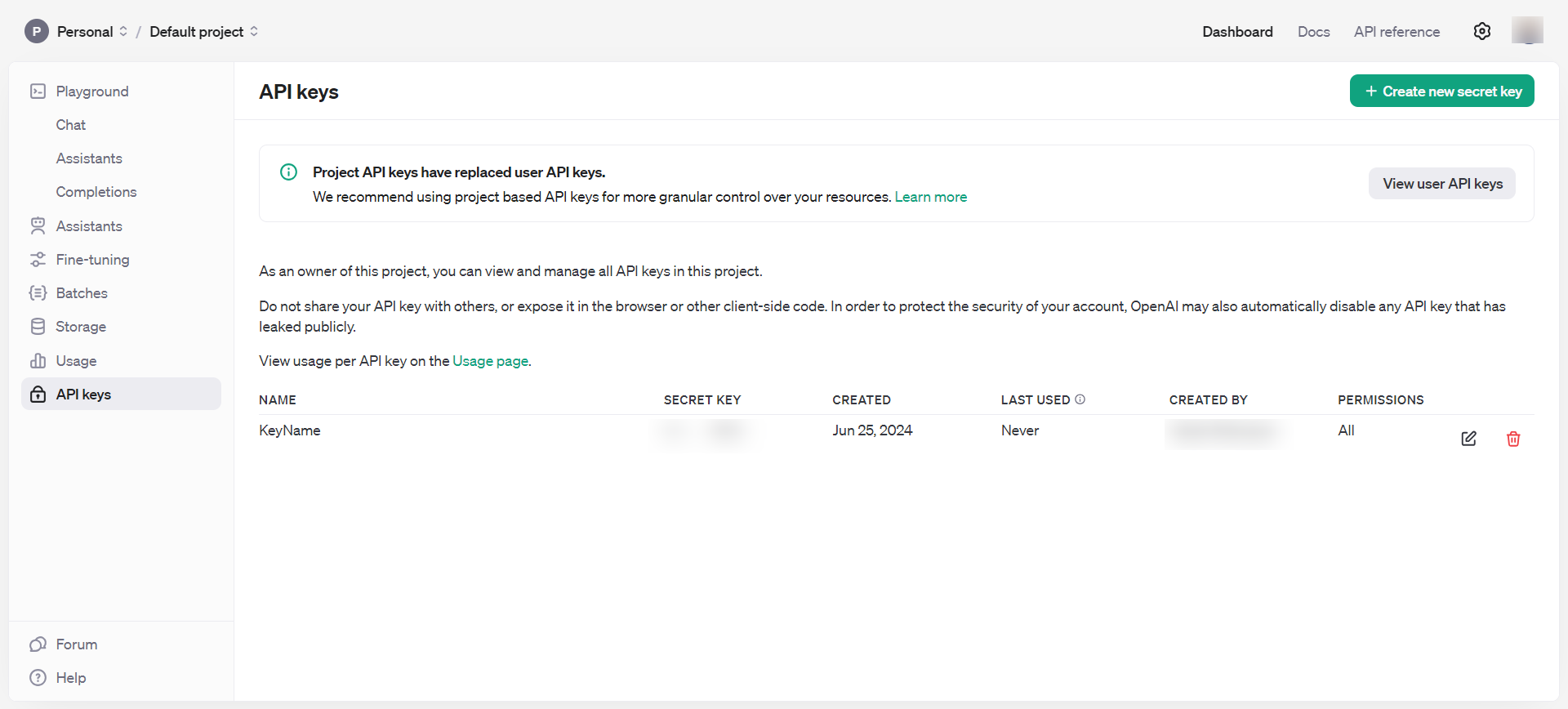 OpenAI API keys
Now, you’ve gotten all the required instruments to start out taking part in with embeddings.
- Open your pc command terminal and sort
jupyter lab. - You must see one thing just like the beneath picture pop up in your browser.
- Click on on Python 3 underneath Pocket book.
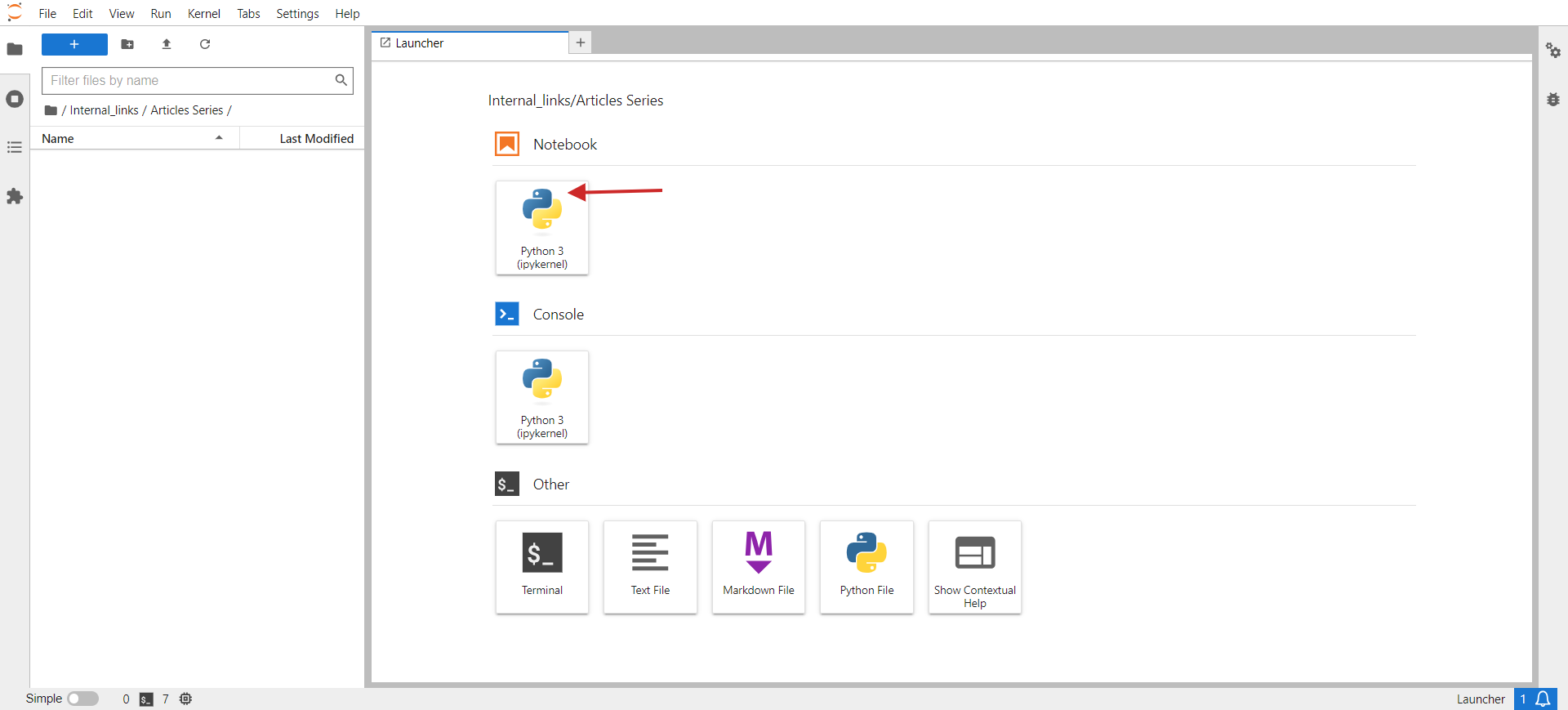 jupyter lab
Within the opened window, you’ll write your code.
As a small job, let’s group related URLs from a CSV. The pattern CSV has two columns: URL and Title. Our script’s job shall be to group URLs with related semantic meanings based mostly on the title so we are able to consolidate these pages into one and repair key phrase cannibalization points.
Listed here are the steps it is advisable to do:
Set up required Python libraries with the next instructions in your PC’s terminal (or in Jupyter pocket book)
pip set up pandas openai scikit-learn numpy unidecode
The ‘openai’ library is required to work together with the OpenAI API to get embeddings, and ‘pandas’ is used for information manipulation and dealing with CSV file operations.
The ‘scikit-learn’ library is important for calculating cosine similarity, and ‘numpy’ is important for numerical operations and dealing with arrays. Lastly, unidecode is used to wash textual content.
Then, obtain the pattern sheet as a CSV, rename the file to pages.csv, and add it to your Jupyter folder the place your script is positioned.
Set your OpenAI API key to the important thing you obtained within the step above, and copy-paste the code beneath into the pocket book.
Run the code by clicking the play triangle icon on the high of the pocket book.
import pandas as pd
import openai
from sklearn.metrics.pairwise import cosine_similarity
import numpy as np
import csv
from unidecode import unidecode
# Perform to wash textual content
def clean_text(textual content: str) -> str:
# First, exchange recognized problematic characters with their right equivalents
replacements = {
'–': '–', # en sprint
'’': '’', # proper single citation mark
'“': '“', # left double citation mark
'â€': '”', # proper double citation mark
'‘': '‘', # left single citation mark
'â€': '—' # em sprint
}
for outdated, new in replacements.gadgets():
textual content = textual content.exchange(outdated, new)
# Then, use unidecode to transliterate any remaining problematic Unicode characters
textual content = unidecode(textual content)
return textual content
# Load the CSV file with UTF-8 encoding from root folder of Jupiter challenge folder
df = pd.read_csv('pages.csv', encoding='utf-8')
# Clear the 'Title' column to take away undesirable symbols
df['Title'] = df['Title'].apply(clean_text)
# Set your OpenAI API key
openai.api_key = 'your-api-key-goes-here'
# Perform to get embeddings
def get_embedding(textual content):
response = openai.Embedding.create(enter=[text], engine="text-embedding-ada-002")
return response['data'][0]['embedding']
# Generate embeddings for all titles
df['embedding'] = df['Title'].apply(get_embedding)
# Create a matrix of embeddings
embedding_matrix = np.vstack(df['embedding'].values)
# Compute cosine similarity matrix
similarity_matrix = cosine_similarity(embedding_matrix)
# Outline similarity threshold
similarity_threshold = 0.9 # since threshold is 0.1 for dissimilarity
# Create an inventory to retailer teams
teams = []
# Maintain monitor of visited indices
visited = set()
# Group related titles based mostly on the similarity matrix
for i in vary(len(similarity_matrix)):
if i not in visited:
# Discover all related titles
similar_indices = np.the place(similarity_matrix[i] >= similarity_threshold)[0]
# Log comparisons
print(f"nChecking similarity for '{df.iloc[i]['Title']}' (Index {i}):")
print("-" * 50)
for j in vary(len(similarity_matrix)):
if i != j: # Be sure that a title isn't in contrast with itself
similarity_value = similarity_matrix[i, j]
comparison_result="better" if similarity_value >= similarity_threshold else 'much less'
print(f"In contrast with '{df.iloc[j]['Title']}' (Index {j}): similarity = {similarity_value:.4f} ({comparison_result} than threshold)")
# Add these indices to visited
visited.replace(similar_indices)
# Add the group to the checklist
group = df.iloc[similar_indices][['URL', 'Title']].to_dict('information')
teams.append(group)
print(f"nFormed Group {len(teams)}:")
for merchandise in group:
print(f" - URL: {merchandise['URL']}, Title: {merchandise['Title']}")
# Examine if teams had been created
if not teams:
print("No teams had been created.")
# Outline the output CSV file
output_file="grouped_pages.csv"
# Write the outcomes to the CSV file with UTF-8 encoding
with open(output_file, 'w', newline="", encoding='utf-8') as csvfile:
fieldnames = ['Group', 'URL', 'Title']
author = csv.DictWriter(csvfile, fieldnames=fieldnames)
author.writeheader()
for group_index, group in enumerate(teams, begin=1):
for web page in group:
cleaned_title = clean_text(web page['Title']) # Guarantee no undesirable symbols within the output
author.writerow({'Group': group_index, 'URL': web page['URL'], 'Title': cleaned_title})
print(f"Writing Group {group_index}, URL: {web page['URL']}, Title: {cleaned_title}")
print(f"Output written to {output_file}")
This code reads a CSV file, ‘pages.csv,’ containing titles and URLs, which you’ll simply export out of your CMS or get by crawling a consumer web site utilizing Screaming Frog.
Then, it cleans the titles from non-UTF characters, generates embedding vectors for every title utilizing OpenAI’s API, calculates the similarity between the titles, teams related titles collectively, and writes the grouped outcomes to a brand new CSV file, ‘grouped_pages.csv.’
Within the key phrase cannibalization job, we use a similarity threshold of 0.9, which suggests if cosine similarity is lower than 0.9, we are going to contemplate articles as completely different. To visualise this in a simplified two-dimensional area, it should seem as two vectors with an angle of roughly 25 levels between them.
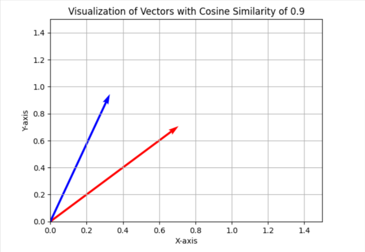
In your case, you might need to use a unique threshold, like 0.85 (roughly 31 levels between them), and run it on a pattern of your information to judge the outcomes and the general high quality of matches. Whether it is unsatisfactory, you possibly can improve the brink to make it extra strict for higher precision.
You may set up ‘matplotlib’ by way of terminal.
And use the Python code beneath in a separate Jupyter pocket book to visualise cosine similarities in two-dimensional area by yourself. Attempt it; it’s enjoyable!
import matplotlib.pyplot as plt
import numpy as np

# Outline the angle for cosine similarity of 0.9. Change right here to your required worth.
theta = np.arccos(0.9)

# Outline the vectors
u = np.array([1, 0])
v = np.array([np.cos(theta), np.sin(theta)])

# Outline the 45 diploma rotation matrix
rotation_matrix = np.array([
    [np.cos(np.pi/4), -np.sin(np.pi/4)],
    [np.sin(np.pi/4), np.cos(np.pi/4)]
])

# Apply the rotation to each vectors
u_rotated = np.dot(rotation_matrix, u)
v_rotated = np.dot(rotation_matrix, v)

# Plotting the vectors
plt.determine()
plt.quiver(0, 0, u_rotated[0], u_rotated[1], angles="xy", scale_units="xy", scale=1, coloration="r")
plt.quiver(0, 0, v_rotated[0], v_rotated[1], angles="xy", scale_units="xy", scale=1, coloration="b")

# Setting the plot limits to solely optimistic ranges
plt.xlim(0, 1.5)
plt.ylim(0, 1.5)

# Including labels and grid
plt.xlabel('X-axis')
plt.ylabel('Y-axis')
plt.grid(True)
plt.title('Visualization of Vectors with Cosine Similarity of 0.9')

# Present the plot
plt.present()
I normally use 0.9 and better for figuring out key phrase cannibalization points, however you might have to set it to 0.5 when coping with outdated article redirects, as outdated articles could not have almost equivalent articles which might be more energizing however partially shut.
It could even be higher to have the meta description concatenated with the title in case of redirects, along with the title.
So, it relies on the duty you’re performing. We are going to assessment the right way to implement redirects in a separate article later on this sequence.
Now, let’s assessment the outcomes with the three fashions talked about above and see how they had been in a position to establish shut articles from our information pattern from Search Engine Journal’s articles.
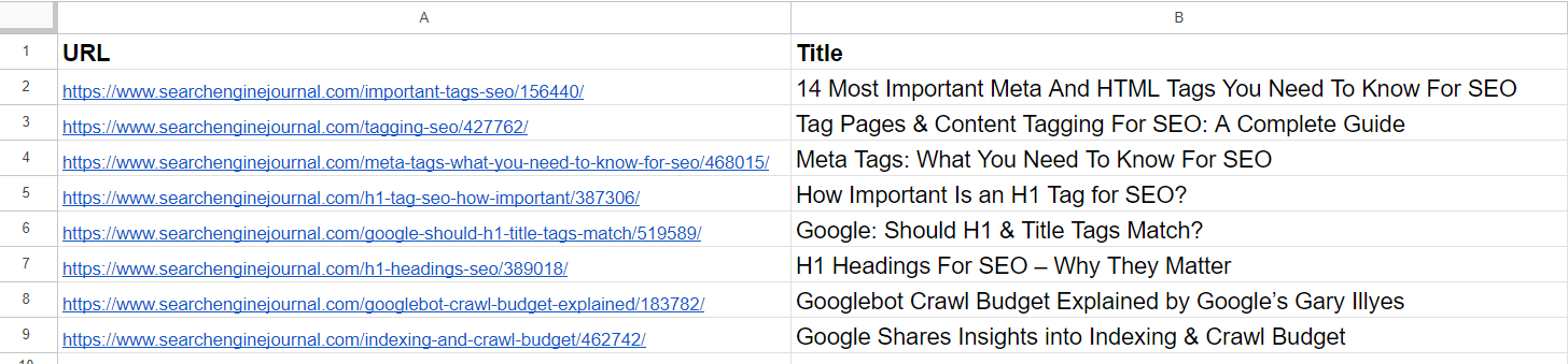 Knowledge Pattern
From the checklist, we already see that the 2nd and 4th articles cowl the identical subject on ‘meta tags.’ The articles within the fifth and seventh rows are just about the identical – discussing the significance of H1 tags in website positioning – and will be merged.
The article within the third row doesn’t have any similarities with any of the articles within the checklist however has frequent phrases like “Tag” or “website positioning.”
The article within the sixth row is once more about H1, however not precisely the identical as H1’s significance to website positioning. As an alternative, it represents Google’s opinion on whether or not they need to match.
Articles on the eighth and ninth rows are fairly shut however nonetheless completely different; they are often mixed.
text-embedding-ada-002
Through the use of ‘text-embedding-ada-002,’ we exactly discovered the 2nd and 4th articles with a cosine similarity of 0.92 and the fifth and seventh articles with a similarity of 0.91.
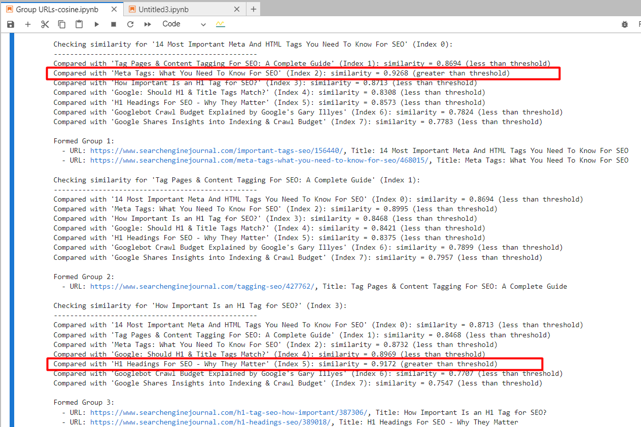 Screenshot from Jupyter log displaying cosine similarities
And it generated output with grouped URLs through the use of the identical group quantity for related articles. (colours are utilized manually for visualization functions).
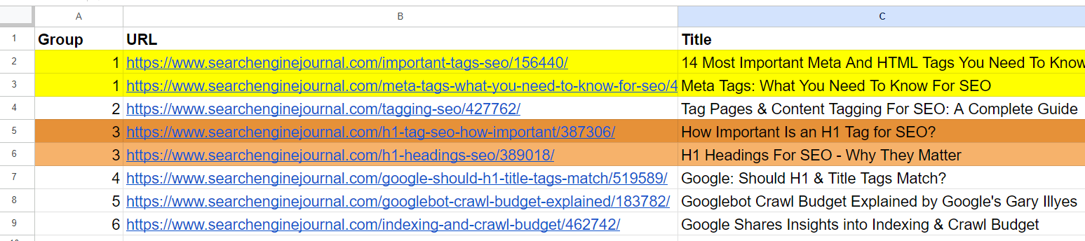 Output sheet with grouped URLs
For the 2nd and third articles, which have frequent phrases “Tag” and “website positioning” however are unrelated, the cosine similarity was 0.86. This exhibits why a excessive similarity threshold of 0.9 or better is important. If we set it to 0.85, it could be filled with false positives and will recommend merging unrelated articles.
text-embedding-3-small
Through the use of ‘text-embedding-3-small,’ fairly surprisingly, it didn’t discover any matches per our similarity threshold of 0.9 or increased.
For the 2nd and 4th articles, cosine similarity was 0.76, and for the fifth and seventh articles, with similarity 0.77.
To higher perceive this mannequin by means of experimentation, I’ve added a barely modified model of the first row with ’15’ vs. ’14’ to the pattern.
- “14 Most Vital Meta And HTML Tags You Want To Know For website positioning”
- “15 Most Vital Meta And HTML Tags You Want To Know For website positioning”
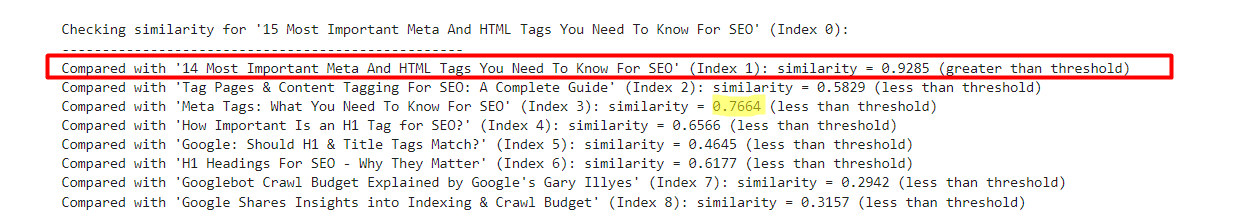 An instance which exhibits text-embedding-3-small outcomes
Quite the opposite, ‘text-embedding-ada-002’ gave 0.98 cosine similarity between these variations.
| Title 1 | Title 2 | Cosine Similarity |
| 14 Most Vital Meta And HTML Tags You Want To Know For website positioning | 15 Most Vital Meta And HTML Tags You Want To Know For website positioning | 0.92 |
| 14 Most Vital Meta And HTML Tags You Want To Know For website positioning | Meta Tags: What You Want To Know For website positioning | 0.76 |
Right here, we see that this mannequin isn’t fairly a great match for evaluating titles.
text-embedding-3-large
This mannequin’s dimensionality is 3072, which is 2 occasions increased than that of ‘text-embedding-3-small’ and ‘text-embedding-ada-002′, with 1536 dimensionality.
Because it has extra dimensions than the opposite fashions, we may anticipate it to seize semantic that means with increased precision.
Nonetheless, it gave the 2nd and 4th articles cosine similarity of 0.70 and the fifth and seventh articles similarity of 0.75.
I’ve examined it once more with barely modified variations of the primary article with ’15’ vs. ’14’ and with out ‘Most Vital’ within the title.
- “14 Most Vital Meta And HTML Tags You Want To Know For website positioning”
- “15 Most Vital Meta And HTML Tags You Want To Know For website positioning”
- “14 Meta And HTML Tags You Want To Know For website positioning”
| Title 1 | Title 2 | Cosine Similarity |
| 14 Most Vital Meta And HTML Tags You Want To Know For website positioning | 15 Most Vital Meta And HTML Tags You Want To Know For website positioning | 0.95 |
| 14 Most Vital Meta And HTML Tags You Want To Know For website positioning | 14 |
0.93 |
| 14 Most Vital Meta And HTML Tags You Want To Know For website positioning | Meta Tags: What You Want To Know For website positioning | 0.70 |
| 15 Most Vital Meta And HTML Tags You Want To Know For website positioning | 14 |
0.86 |
So we are able to see that ‘text-embedding-3-large’ is underperforming in comparison with ‘text-embedding-ada-002’ after we calculate cosine similarities between titles.
I need to be aware that the accuracy of ‘text-embedding-3-large’ will increase with the size of the textual content, however ‘text-embedding-ada-002’ nonetheless performs higher general.
One other method could possibly be to strip away cease phrases from the textual content. Eradicating these can typically assist focus the embeddings on extra significant phrases, probably enhancing the accuracy of duties like similarity calculations.
One of the simplest ways to find out whether or not eradicating cease phrases improves accuracy in your particular job and dataset is to empirically check each approaches and examine the outcomes.
Conclusion
With these examples, you’ve gotten discovered the right way to work with OpenAI’s embedding fashions and might already carry out a variety of duties.
For similarity thresholds, it is advisable to experiment with your personal datasets and see which thresholds make sense in your particular job by working it on smaller samples of knowledge and performing a human assessment of the output.
Please be aware that the code we’ve on this article isn’t optimum for giant datasets since it is advisable to create textual content embeddings of articles each time there’s a change in your dataset to judge in opposition to different rows.
To make it environment friendly, we should use vector databases and retailer embedding data there as soon as generated. We are going to cowl the right way to use vector databases very quickly and alter the code pattern right here to make use of a vector database.
Extra sources:
Featured Picture: BestForBest/Shutterstock

